DE WITT
|
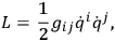
where the
 may be functions of the
 ’s and the indices
 run from
 to
to
 . The
fact that
. The
fact that
 may be nondenumerably infinite is ignored. For an actual system the Lagrangian may possess other terms, but the essential difficulties are contained in the term considered. Inclusion of the other terms modifies the following discussion in no essential way.
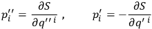
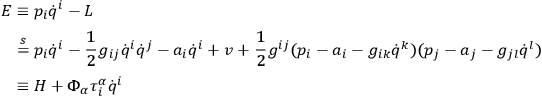
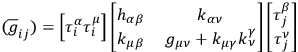
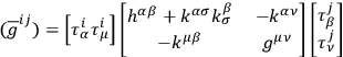
If (
 ) is a nonsingular matrix with inverse given by (
 ) then the system possesses a Hamiltonian function given by
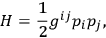
|
and the action
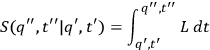
|
satisfies the Hamilton-Jacobi equations
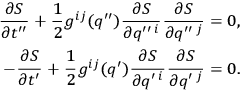
|
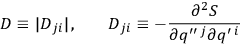
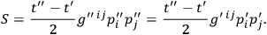
According to DE WITT, , which is already contained in the Lagrangian to be taken as the metric for the space of the
 ’s and provides the appropriate “measure” for a Feynman summation.
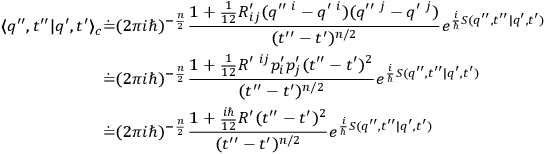
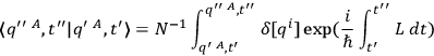
Following Pauli1 one may introduce a “classical kernel” of the form
’s and provides the appropriate “measure” for a Feynman summation.
Following Pauli1 one may introduce a “classical kernel” of the form

|
where
 , and where the quantity
 is a determinant originally introduced by Van Vleck in an attempt to extend the WKB method to systems in more than one dimension.2
|
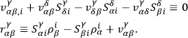
and satisfies an important conservation law:
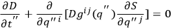
|
which can be obtained by differentiating the first Hamilton-Jacobi equation with respect to
 and
and
 and multiplying by the inverse matrix
 . From the quantum viewpoint this law expresses conservation of probability.
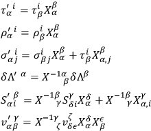
It is easy to see that
 is an invariant under point transformations of the
 ’s. With the aid of the Hamilton-Jacobi equations one may show that
it satisfies the differential equations
’s. With the aid of the Hamilton-Jacobi equations one may show that
it satisfies the differential equations
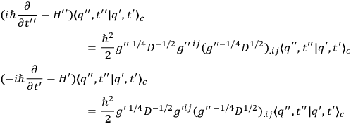
|
where for brevity we write
 , etc.; where the dot followed by indices denotes covariant differentiation with respect to either the
 or
or
 (as indicated by the context) and where the operator
 is defined by
|
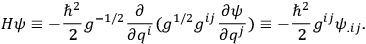
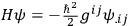
DE WITT  ’s is curved, the operator
 could immediately
be regarded as the Hamiltonian operator for the quantized system. In order to discuss this phenomenon some further development is necessary:
could immediately
be regarded as the Hamiltonian operator for the quantized system. In order to discuss this phenomenon some further development is necessary:
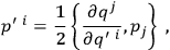
If one recalls that the classical action defines a canonical transformation by the equations
|
then one easily sees that the Van Vleck determinant is just the Jacobian involved in transforming from a specification of the classical path by means of the variables
 ,
,
 , to a specification in terms
of initial variables
, to a specification in terms
of initial variables
 ,
,
 . From the Hamilton-Jacobi equations one sees furthermore that the action may be expressed in the form
|
Therefore, noting that as
 the
the
 become infinite except when
 (for all
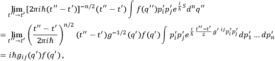
 ), one may write, for an arbitrary function
 ,
,
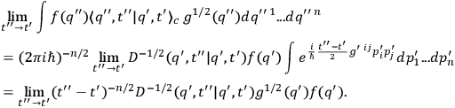
|
In order to evaluate this last expression one must evaluate the Van Vleck determinant. This is easily done by expanding the action about the point substituting it in the Hamilton-Jacobi equation. One finds, after a straightforward computation,
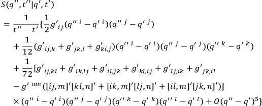
|
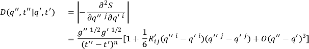
|
where
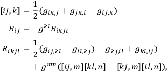
|
commas followed by indices denoting differentiation with respect to the
 ’s. Here a convention has been chosen so that the scalar
 is positive for a space of positive curvature.
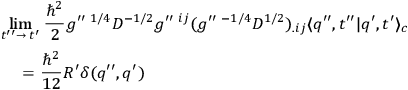
Using the final expression for the Van Vleck determinant one infers
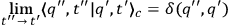
|
and
|
where
 is the invariant delta-function in
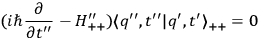
 -space. Referring to the differential equations satisfied by the classical kernel
 , one sees that it equals the true quantum transformation function
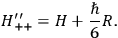
 of a system possessing the Hamiltonian operator
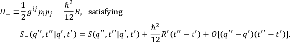
|
up to the first order in
 . That is,

|
where
|
satisfying the boundary condition

|
The “first order contact” between
 and
and
 is already
sufficient to determine the behavior of wave packets for the quantized system. If the system has a Hamiltonian operator
is already
sufficient to determine the behavior of wave packets for the quantized system. If the system has a Hamiltonian operator
 then its wave packets will more approximately along the classical paths of a classical system which has simply
 as Hamiltonian function. Conversely if the quantized system has Hamiltonian operator
 then the motions of its wave packets will be along the classical paths for a “classical” system which has the Hamiltonian function
 . Evidently there is an ambiguity here in the choice of Hamiltonian operator when the space is curved, and there is nothing in the classical theory to resolve it for us.
The Feynman formulation of quantum mechanics follows immediately from the order contact between
 and
and
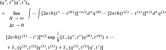
 . Breaking the transformation function up into infinitely many pieces by means of the composition law

|
where
 , one may write
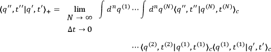
|
where
 . It is evident, from the expression for
 and the form of the expansion for the action
 , that the (in the limit) infinitely multiple integral receives significant contributions from the integrand only when the differences
 are of the order of
 or smaller. Therefore, if the symbol
 is used to denote equivalence as far as use in the infinitely multiple integral is concerned, one may write
|
since
|
and therefore

|
where
 is the action function for the system with classical Hamiltonian function
|
The Feynman formulation now becomes
|
and the dependence of the “sum-over-paths” on the metric
 is seen to occur through the invariant volume elements
 . This last expression is sometimes written in the symbolic form
|
where the symbol
 indicates that a “functional integration”
  .
.
It will be noted that the last result is even more curious than the previous result obtained with the Pauli method using
 . In order to obtain the transformation function for a quantized system having Hamiltonian operator
 one must use, in the Feynman summation, the action corresponding to a classical system
having Hamiltonian
one must use, in the Feynman summation, the action corresponding to a classical system
having Hamiltonian
 or Lagrangian
 . When DE WITT
  actually cancelled each other when one passed from the Pauli form on to the Feynman representation. J. L. Anderson later convinced him, however, of the reality of the phenomenon, by carrying out a computation patterned directly after Feynman's original paper.
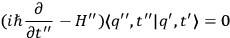
Instead of stating the result in a symmetric manner one may also state it in the following forms: If the true classical action
 is used in the Feynman summation then one generates the transformation function
 satisfying
|
where
|
On the other hand, in order to generate the transformation function
 satisfying
|
one must use in the Feynman summation the action for a “classical” system possessing the Lagrangian function
|
and Hamiltonian function
|
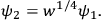
FEYNMAN remarked that quantization of a system like
 is necessarily ambiguous when the space is curved.
DE WITT
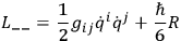
Fig. 21.1
In order to eliminate, right at the start, the degree of freedom transverse to the shell - which must have no reality in the end, anyway - one may suppose that the wave function has a simple node on each ellipsoid and none in between (i. e., transverse ground state). Since we know that confocal ellipsoids form a separable system for Schrödinger equation, we may immediately factor out the transverse part of the wave function and at the same time subtract a constant term proportional to
 from the energy, where
 denotes the thickness of the shell at some point. The remaining part of the wave function then satisfies the Schrödinger equation with the simple operator
 appropriate to an ellipsoid. This corresponds to a Feynman formulation using the classical Lagrangian
 , for which the classical paths are attracted
to the region of greatest positive curvature, the attraction being described by a potential
, for which the classical paths are attracted
to the region of greatest positive curvature, the attraction being described by a potential
 . In the present case the region of greatest positive curvature is the “nose” of the ellipsoid and here the shell is thinnest. The
three-dimensional wave function undergoes a “crowding” at this point. Since the transverse part of the wave function is constant, this crowding must be borne by the
“active” two-dimensional part. The tendency of the amplitude to increase in the nose region is describable in classical terms as an attraction. A wave packet would
actually display the effect of this attraction.
. In the present case the region of greatest positive curvature is the “nose” of the ellipsoid and here the shell is thinnest. The
three-dimensional wave function undergoes a “crowding” at this point. Since the transverse part of the wave function is constant, this crowding must be borne by the
“active” two-dimensional part. The tendency of the amplitude to increase in the nose region is describable in classical terms as an attraction. A wave packet would
actually display the effect of this attraction.
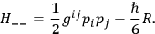
The Feynman formulation which starts with the classical Lagrangian
 , on the other hand, corresponds to the use of a shell of uniform thickness:
Fig. 21.2
All points of the limiting ellipsoid are here weighted equally. DE WITT  .
.
(Editor's Note: - DE WITT's argument is not entirely rigorous. He, of course, avoided discussion of a spherical shell since the curvature is then constant and has only the effect of uniformly shifting all energy levels. However, there is a difficulty for ellipsoidal systems in that the separation constants are not themselves separable, and hence the transverse part of the wave function is not rigorously factorable for arbitrary behavior of the non-transverse part. It may, however, be approximately factorable when the shell is thin.
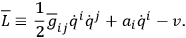
Attention should also be called to the fact that the behavior of wave packets is not described by the Lagrangian appearing in the Feynman formulation but by the
Lagrangian of the Pauli formulation, which is half-way between that of Feynman and the corresponding quantum form. Thus, when Feynman uses
 , Pauli uses
 to obtain the same quantum theory. Or when Feynman uses
 , Pauli uses
 . It is the Van Vleck determinant of the Pauli formulation which gives the key to the motion of wave packets, through its conservation law. Remembering that
 , one may write that conservation law in the form
|
If a wave packet is replaced by an ensemble of classical particles then
 gives a measure of the density of these particles at any time and place.)
WHEELER
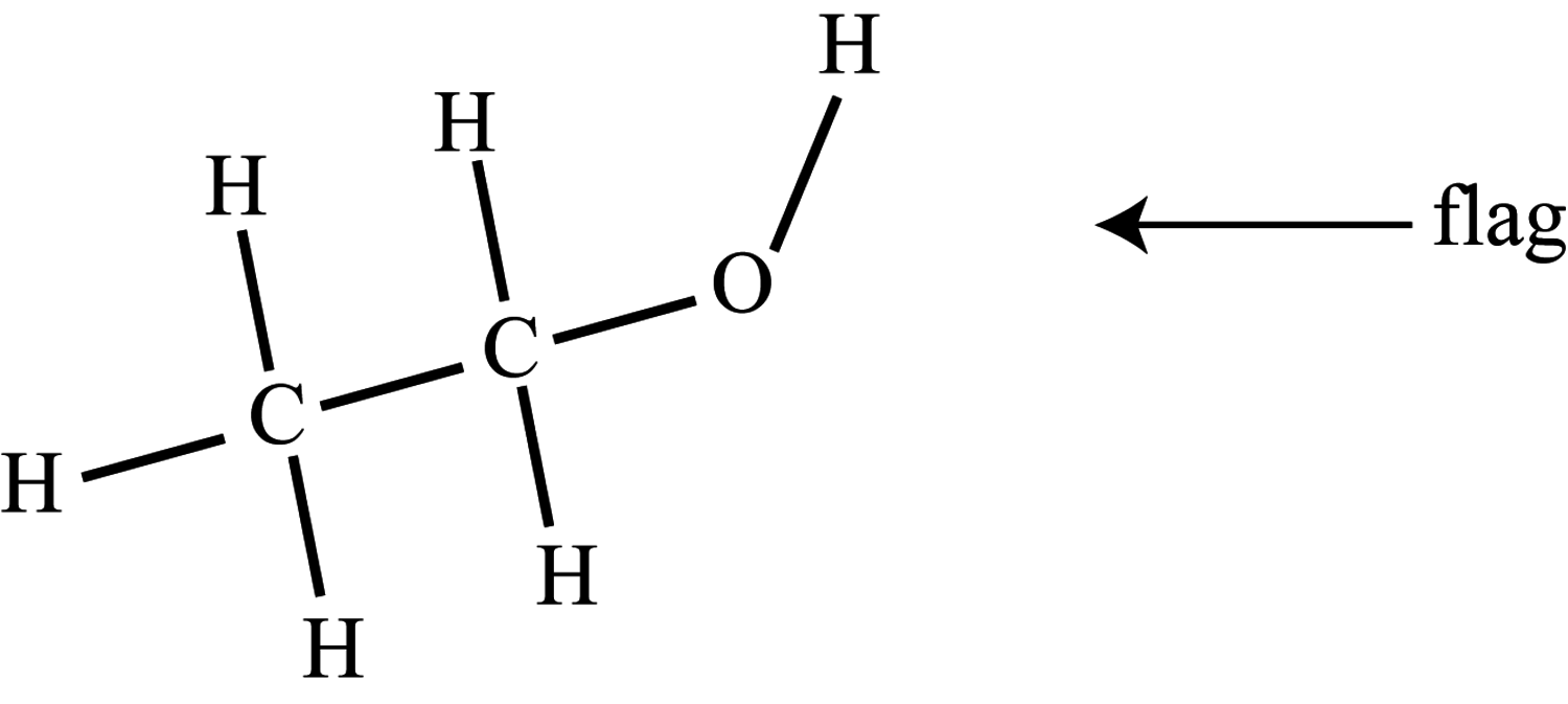
Fig. 21.3
If some of the bonds are regarded as rigid (e.g., at room temperature) then the Lagrangian for such a molecule contains a metric corresponding to a space which is
not flat. However, WHEELER
ANDERSON . This relation will not generally be satisfied if one chooses a metric for
 -space which is unrelated to the
 appearing in the Lagrangian.
DE WITT then went on to discuss the second important and pressing problem which arises in the quantization of nonlinear systems, namely, the “factor ordering problem”: How should one order non-commuting operators to obtain appropriate quantum analogs of various classical equations?
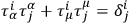
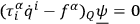
When the matrix (
 ) is non-singular the factor ordering
Hamiltonian operator is easily solved. The Hermitian requirement on the momenta
) is non-singular the factor ordering
Hamiltonian operator is easily solved. The Hermitian requirement on the momenta
 leads to the quantum representation requirement
|
in arbitrary curvilinear coordinates. Hence, in order that
 , one must write
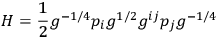
|
The Hermitian character of
 is obvious from the symmetry of this expression.
For covariant theories, on the other hand,
 is singular, constraints
  is singular it is not obvious immediately what “measure” to use in a Feynman formulation.
(Editor's Note: - The following is taken from a set of mimeographed notes which DE WITT
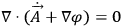
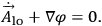
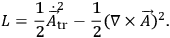
As a prototype of a covariant theory DE WITT
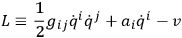
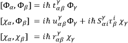
|
for which the equations of motion are

|
where
 . These equations of motion are, of course, invariant under point transformations of the
 's among themselves as well as under “phase transformations”
 where
where
 is an arbitrary function of the
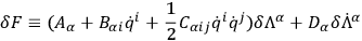
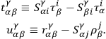
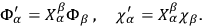
 's, The “covariance” of the theory is described by an additional transformation group under which the equations of motion remain invariant, whose infinitesimal elements have the general form
 , where

|
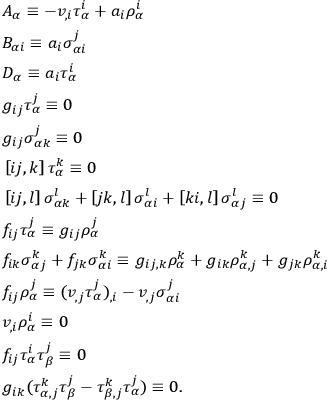
The
 ,
,
 ,
,
 are certain definite functions of the
 's, while the
 are arbitrary infinitesimal functions of the time and of the
 's and any of their time derivatives. Such a transformation may be called a gauge transformation; in general relativity it is an infinitesimal coordinate transformation, the
 being the metric field variables.
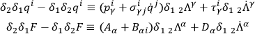
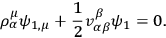
The Lagrangian function must be altered under a gauge transformation by a total time derivative
 . It is not hard to see that
 must have the general form
|
where the
 ,
,
 ,
,
 ,
,
 are functions of the
 's only. DE WITT
  , as this simplifies the analysis in certain respects. This assumption is actually incorrect for the gravitational field, but is not expected to alter the main qualitative features of the analysis. (It will be discussed more fully at a later point.) By performing a gauge transformation on the Lagrangian and making a comparison with
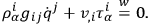
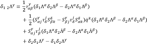
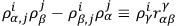
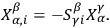
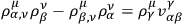
 one finds that the following identities must be satisfied:
|
DE WITT
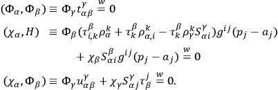
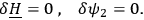
It is the identity
 which shows that (
 ) must be a singular matrix in a “gauge invariant” theory. This has the consequence that the momenta of the Hamiltonian formalism are not all independent. It also has the consequence that the initial conditions on the motion must be subject to constraints
  an extremum. Some, at least, of these constraints are obtained by multiplying the equations of motion by
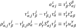
 . Using identities of invariance one finds
|
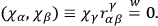
These will constitute the complete set of constraints
DE WITT  form a complete and independent set of null eigenvectors of
 . One may then infer that
|
where the
 ,
,
 ,
,
 are certain coefficients. DE WITT
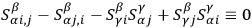
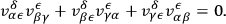
A final set of identities are obtained from the group property of gauge transformations. Requiring that the difference between the results of applying two infinitesimal gauge transformations in different orders be also a gauge transformation (of the second infinitesimal order) one finds
|
where
|
only if
|
for certain coefficients
 , and if
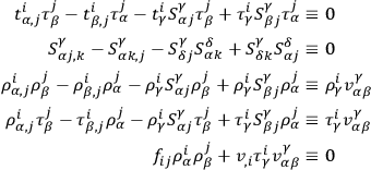
|
where the
 are certain coefficients satisfying
|
DE WITT
|
DE WITT  ) and strong equations (
 ). Equations of motion and constraints
  ) are strong equations. Also, the product of two weakly vanishing functions is strongly equal to zero.
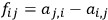
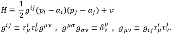
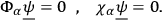
The canonical momenta for the system are
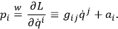
|
Multiplication by
 gives immediately the set of constraints
|
Completing the set of vectors
 through the introduction of a set of independent vectors
 , and introducing also “inverses”
 ,
,
 satisfying
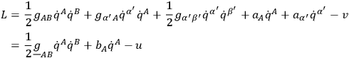
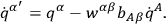
 , one may write the “energy function” in the form
|
where
|
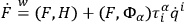
The final expression for the energy function provides an illustration of Dirac's theorem  of the
 's and
 's, which may be called the Hamiltonian function, plus a linear combination of the
 's with coefficients which depend on the velocities
 . In a theory without constraints the energy is identical with the Hamiltonian function. When constraints are present the two are only weakly equal.
If the coefficients multiplying the
 's are completely undetermined by the equations of motion, and hence completely arbitrary, the
 's are said to be “of the first class.” This point always requires special investigation. Using the equations of motion together with the constraints
  of the
 's and
 's is given by
|
where
 denotes the Poisson bracket. In particular, the time rate of change of a
 is given by
|
Since the
 's vanish their time derivatives must also vanish. This will happen automatically if the Poisson brackets
 and
and
 vanish, at least weakly. If these Poisson brackets do not all vanish then the
 cannot all be completely arbitrary and the
 will be subject to additional constraints.
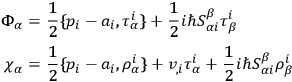
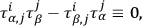
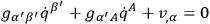
Using the relation
 together with identities of invariance, one finds, after a straightforward computation,

|
where
|
The latter equations are simply the velocity constraints  -equations, existing only in the canonical formalism, are sometimes known as “primary constraints.” The
 -equations, which follow from them, are then called “secondary constraints.” The
 's as well as the
 's must have vanishing time
derivatives. This leads one to investigate also the Poisson brackets
's must have vanishing time
derivatives. This leads one to investigate also the Poisson brackets
 .
.
Using only the identities of invariance and completeness one finds
|
The vanishing (in the weak sense) of all these Poisson brackets means that
there exist no further constraints  's are all of the first class. There still remains, however, one further Poisson bracket which it is necessary to examine, namely
 . Dirac
In the evaluation of
 identities of integrability are needed for the first time. One finds
|
Evidently Dirac brackets are here the same as ordinary Poisson brackets. Under these circumstances the
 's are said to be “of the first class.” It is characteristic of any theory in which the constraints
  's and
 's are of the first class.
DE WITT
DE WITT  and
and
 equations, which, in the quantum theory, are to be regarded as supplementary conditions on the state vector
 of the system:
|
Since the classical expressions for the
 and
and
 involve quantities which, in the quantum theory, do not commute, the factor ordering problem here makes its appearance. According to DE WITT
  and
and
 should be taken as
|
where
 denotes the anticommutator bracket. With the aid of the previously unused identities of integrability one may then show that
|
where
 denotes the commutator bracket and where the ordering of factors
on the right is now important. Since the
denotes the commutator bracket and where the ordering of factors
on the right is now important. Since the
 's and
 's all stand to the extreme right the corollaries

|
of the supplementary conditions are automatically satisfied. DE WITT  above) which are proportional to
 or powers of
 , and which do not appear in the corresponding classical expression (since
 ).
).
Similar considerations are involved in finding the quantum analog of the
function
 . It is convenient to return for a moment to the classical theory: Since the
 's and
 's are all of the first class, the quantities
 appearing in the dynamical equation (i.e., for
 ) are completely arbitrary. One is at liberty to set them equal to arbitrary functions
 of the
 's and
 's through the addition of
extra supplementary conditions:
's through the addition of
extra supplementary conditions:

|
The energy function
 is then strongly equal to
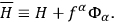
|
Furthermore, the dynamical equation may be replaced by

|
The conditions
 ,
,
 are, of course, unaffected.
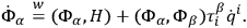
In the quantum theory the dynamical equation may be taken as

|
in which the quantum form of
 is written as above with the
 's standing to the right. The time derivatives of the supplementary conditions, namely
|
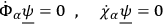
will then be satisfied provided

|
The quantum form of
 will be chosen in such a way that these equations are automatically satisfied by virtue of the supplementary conditions. The supplementary
conditions when combined with the dynamical equations for
will be chosen in such a way that these equations are automatically satisfied by virtue of the supplementary conditions. The supplementary
conditions when combined with the dynamical equations for
 will generally imply

|
where
 indicates some suitable quantum analog for
 , and in this way the consistency of the quantum scheme can be checked for arbitrary choices of the
 .
.
It is to be noted that one is here working in the Heisenberg picture in which the state vector
 is time independent. The arbitrariness in the choice of
the functions
is time independent. The arbitrariness in the choice of
the functions
 shows that there are many different Heisenberg pictures, all equally valid. They all lead, however, to a single unique Schrödinger picture:
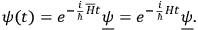
|
One may arrive directly at the Schrödinger picture by starting, in the classical theory, from the “homogeneous velocity” formalism (Dirac,  . This leads to a new
 equation, namely
 where
where
 . In the quantum theory, representation of

 puts the corresponding condition on the state vector in the form

|
which is just the Schrödinger equation.
Construction of the quantum form of
 is more difficult than the construction of the quantum forms of
 and
and
 for two reasons: (1)
 is quadratic rather than linear in the momenta. (2) No metric has yet been defined in
 -space. If there were no gauge transformation group for the system,
 would be nonsingular and
would, as DE WITT
would be nonsingular and
would, as DE WITT  as a sort of superstructure with
 as a core, in the following manner:
|
matrix multiplication as indicated, where
 ,
,

 are arbitrary functions of the
 's. However,
 is assumed to have an inverse
 which is used to raise the indices
 ,
,
 ,
,
 , etc., while
 is used to raise the indices
 ,
,
 ,
,
 , etc. (
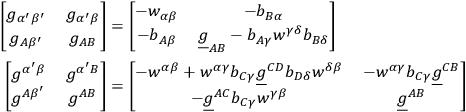
 ) will then have an inverse given by
|
and a determinant given by

|
where
 ,
,
 ,
,
 . The metric
 may be used to make a special choice for the function
 , namely
|
corresponding to the choice

|
The equations of motion generated by this “Hamiltonian” may be derived from a Lagrangian function of the form
|
The quantum theory generated by this Lagrangian function is not identical with that which has been developed here, but becomes so upon the addition of the equations
 as supplementary conditions. This is a standard procedure in quantum electrodynamics in which these supplementary conditions become the “Lorentz
conditions.”
as supplementary conditions. This is a standard procedure in quantum electrodynamics in which these supplementary conditions become the “Lorentz
conditions.”
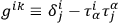
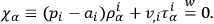
A choice of metric having been adopted, one may now express the quantized momenta explicitly in the form
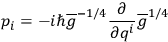
|
and one finds that the supplementary conditions become
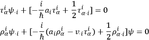
|
a dot followed by an index denoting covariant differentiation with respect to the metric
 , with, however, the modification
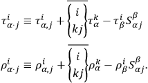
|
 being the Christoffel symbol
  . A special significance possessed by the coefficients
 is here emphasized. The
 provide a kind of affine connection in terms of which one may define parallel displacements which are invariant not only under point transformations but also under transformations associated with the indices
 ,
,
 , etc., of the form
|
where the
 are arbitrary functions of the
 's, the matrix (
 ) possessing, however, an inverse (
 ). These transformations, which DE WITT
  -transformations, leave all the identities of invariance, completeness, and integrability unchanged. The
 -transformation procedure may be extended to the indices
 ,
,
 ,
,
 , etc., by the definitions
|
where the
 ,
,
 are also arbitrary functions of the
 's, with (
 ) possessing as an inverse (
 ). The whole theory (in particular, the metric
 ) will then
be invariant under
) will then
be invariant under
 -transformations provided
|
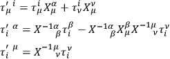
In order to show the invariance of the quantum theory under point, phase, gauge, and
 -transformations one does not actually have to use the differential representation of the momenta, convenient though it generally is. For example, the
point transformation law for the momenta is
-transformations one does not actually have to use the differential representation of the momenta, convenient though it generally is. For example, the
point transformation law for the momenta is
|
and, remembering that the indices
 etc., on the quantities
 ,
,
 ,
,
 ,
,
 ,
,
 ,
,
 , etc., are all tensor indices under point transformations, one finds by
straightforward computation that
, etc., are all tensor indices under point transformations, one finds by
straightforward computation that
 ,
,
 ,
,
 , provided one writes

|
where
 is a scalar function of the
 's, as yet undetermined. Similarly, under
 -transformations one finds
 and
and
|
Since the
 's and
 's stand to the right the supplementary conditions remainunchanged:
 ,
,
 . Invariance of the quantum theory under gauge
transformations is not immediately apparent at this point, but becomes so subsequently. Phase transformations, on the other hand, are trivial:
. Invariance of the quantum theory under gauge
transformations is not immediately apparent at this point, but becomes so subsequently. Phase transformations, on the other hand, are trivial:

|
or, if one is using the fixed differential representation for the momenta, one places the burden of keeping the theory phase-invariant on the state vector (or wave function) by the law

|
Having introduced
 -transformations, DE WITT
  satisfies the very important condition of being integrable. This
means that one can carry out an
satisfies the very important condition of being integrable. This
means that one can carry out an
 -transformation which will make the
 vanish everywhere. The required transformation is given by the solutions of the simultaneous equations
|
The solubility of these equations is guaranteed by the identity of integrability
 . After this transformation has been carried out one has
|
which implies that there exists a point transformation
 such that

|
Making this point transformation, together with an additional
 -transformation

|
and letting the
 be given by

|
one arrives at a great simplification in the formalism. Using a simple replacement of indices
 ;
;
 , etc., to denote quantities in the new “coordinate system,” one has
|
Moreover, the identities of invariance and integrability take the forms
|
The identity
 implies that a phase transformation (
 ) can be
carried out which makes
) can be
carried out which makes
 vanish. Assuming that it has already been performed and noting that
|
one may now write the supplementary condition in the forms
|
The first supplementary condition has the important result that the arbitrary quantities
 can now be actually eliminated entirely from the quantum theory, just as they are not needed in the classical theory. That is, having carefully built up a “superstructure” around the metric
 (or
(or
 ), one then proceeds to throw it away. To do this one simply introduces a new wave function
|
This definition removes from the wave function that part of the metric density which refers exclusively to the
 , and corresponds to the use of
 as invariant volume element. The condition
 means that the new wave function does not depend on the variables
 . The
. The
 are non-observable or “non-physical” variables of the system. This was, in fact, already true in the classical theory, since the
 can be made to undergo arbitrary changes by means of gauge transformations.
In the new representation
 by itself provides a natural metric in the reduced space of the
 . To see how this works for the Hamiltonian operator, one can multiply the Schrödinger equation

|
by
 . Using the explicit form for
 , one finds, after a straightforward calculation,

|
where the dots now denote covariant differentiation with respect to the metric
 , and where

|
The quantity
 is invariant under point transformations which are restricted to the variables
 alone.
The new Schrödinger equation may be written in the form

|
where

|
the explicit differential form for the momenta
 in the new representation being
|
The existence of the second supplementary condition suggests that there are further non-physical variables in addition to the
 . To show this one must first
eliminate the term in
. To show this one must first
eliminate the term in
 from the supplementary condition. This can be done by carrying out a phase transformation
 satisfying

|
and at the same time satisfying

|
so as not to disturb the condition
 . The integrability of these equations is insured by the identities of invariance and integrability, as one may verify by
straightforward computation, showing that the expressions for
. The integrability of these equations is insured by the identities of invariance and integrability, as one may verify by
straightforward computation, showing that the expressions for
 and
and
 vanish. One may then write
|
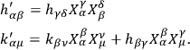
Next, by differentiating the identity
 one can show that
|
The coefficients
 are then immediately recognizable as the structure constants
of a Lie group. The secondary constraints
are then immediately recognizable as the structure constants
of a Lie group. The secondary constraints  are, in fact, the infinitesimal generators of the group. In the general case the structure constants will be
non-vanishing and the Lie group will be non-Abelian. This immediately leads one to various possibilities depending on the classification of the Lie group in question. As an illustration, suppose that the Lie group is the irreducible rotation group in
are, in fact, the infinitesimal generators of the group. In the general case the structure constants will be
non-vanishing and the Lie group will be non-Abelian. This immediately leads one to various possibilities depending on the classification of the Lie group in question. As an illustration, suppose that the Lie group is the irreducible rotation group in
 dimensions. The indices
 must then range over
 different values. This is not however the number of further non-physical variables. A point transformation
 can
be made such that the new variables
can
be made such that the new variables
 describe the subspace in which the rotations actually take place. The quantity
 vanishes for the rotation group and the second supplementary condition is found to reduce to
 which, when analyzed, is seen to state simply that the wave function is invariant under rotations in the subspace of the
 . Therefore, in this case only
 further variables can be eliminated from the theory as non-physical. The wave function can still depend on the rotation-invariant combination
 as well as on the
 .
.
The primary constraints  also, of course, generate a Lie group. But this group is necessarily Abelian.
DE WITT
also, of course, generate a Lie group. But this group is necessarily Abelian.
DE WITT  is also Abelian (so that
 ) and furthermore that the vectors
 are linearly independent of the
 and of each other. In this case, when
 , one may carry out a point transformation
 such that
|
(Here, in order to avoid confusion one must use a prime to distinguish indices related to the
 from those related to the
 .) In the new “coordinate system” one has
|
and the identities of invariance and integrability become
|
If the phase is adjusted so that
|
then one also has
|
Moreover, the supplementary conditions become
|
so that the
 , like the
 , are now “non-physical” variables.
The quantity
 is seen to be independent of the
 and to have a dependence on the
 which is no more than quadratic (since
 ). One may choose the origin of the unobservable “coordinates”
 in such a way that
|
where
 and
and
 are independent of the
 and
and
 . Furthermore, since
 and
and
 , one may write
|
where
 and
and
 are independent of the
 and
and
 . In order to complete the elimination of the
 from the theory, a natural metric
 for the reduced space of the
 must be introduced. DE WITT showed that it must be defined in the following manner:
|
in which use has been made of the relations
 ,
,
 , and in which the matrix (
 ) is assumed to have an inverse (
 ).
).
With this definition one has
 and
and

|
where
 and
and
 . The determinant
 forms that part of the metric density
 which refers exclusively to the non-physical variables
 . It may be removed from the normalization of the wave function
 by introducing a new wave function
|
Since
 ,
,
 ,
,
 is independent of the
 and
and
 . It may becalled the “true physical wave function” of the system referring only to the “physical” variables
 . Its Schrödinger equation may be found by multiplying the
Schrödinger equation
. Its Schrödinger equation may be found by multiplying the
Schrödinger equation
 by
by
 making use of the relations
|
One finds, after a straightforward computation,

|
where
|
The operator
 remains invariant under point transformations which are restricted to the variables
 alone.
The operators
 ,
,
 and any quantities constructed out of them are the true observables
|
One has only to require that
 be independent of the
 and
and
 .
.
 will then be a true observable
 and
and
 ) and the wave function
 will remain independent of the
 and
and
 at all times.
The gauge invariance of the quantum theory is now also
immediately evident. In the “coordinate” system
 ,
,
 ,
,
 , gauge transformations are given simply by

|
and hence
|
There remains only the term
 which is unknown. However this term, as Feynman
 in the limit, and this is arbitrary.
It is of interest to examine the Feynman quantization only, using the measure defined by the metric
 . The variables
 may be chosen as arbitrary functions of the time (corresponding to the original arbitrariness in the
 ) and the original Lagrangian function
 may be used to compute the action, provided the variables
 are made to vary in time in such a way as to satisfy the velocity constraints
|
or
|
For the Lagrangian function then becomes
|
which is precisely the form which gives rise to the Hamiltonian
 . One may therefore express the transformation function in the symbolic form
|
with the understanding that the functional integration  and
and
 which satisfy the velocity constraints
  given, each path being assigned a weight according to the measuredefined by
 . (Here, potential-like terms proportional to
 , which may be added to
 , are ignored.)
It is not actually necessary to restrict the summation to the variables
 only. For example, one may work with the transformation function
|
which connects the values of the wave function
 at two different times. Since
 is independent of the
 for physical states, one may write
|
which implies

|
The expression on the right must be independent of the
 . Hence one may integrate over these variables provided one divides the result by an infinite normalization factor. Moreover, in the path summation expression for
 the choice of time-like behavior for the variables
 is immaterial. Hence one may write
|
where
 is a suitable infinite normalization factor, the functional integration
  ,
,
 at
at
 ,
,
 respectively (all possible end-point values for the variables
 ,
,
 being included in the summation) each path being given a weight according to the measure defined by metric density
 multiplied by the Jacobian of the transformation
 ,
,
 ,
,
 . In calculation of actual physical quantities one never needs to mention the normalization factor
 explicitly, since what is involved is always a ratio of the form
|
where
 is some true observable
 ,
,
 alone), and the normalization factors in front of the functional integrals cancel.
DE WITT  , occurring in the expression for
 , vanish. In the case of the Lagrangian for the gravitational field the
 do not vanish. This has the result that the secondary constraints
  are no longer linear in the momenta, but quadratic. In fact, it had been pointed out earlier in the conference that the quadratic term, in the gravitational case, is just the energy density for the gravitational field. This created a certain amount of perplexity, leading some of the participants to think that perhaps all true observables
 will be considerably more difficult in the case
 .
The resulting quadratic dependence of the
.
The resulting quadratic dependence of the
 on the momenta means that the non-physical variables can no longer be found simply by a point transformation. A more complicated type of canonical transformation will be required.
DE WITT suggested that the use of parametrized space-like surfaces might help this situation. But he also pointed out that the equations like
 become variational differential equations
in field equations in field theories, and that there is some uncertainty about the ease with which they can be solved in nonlinear contexts. The search for answers to these questions will provide a large program for the future.
become variational differential equations
in field equations in field theories, and that there is some uncertainty about the ease with which they can be solved in nonlinear contexts. The search for answers to these questions will provide a large program for the future.
FEYNMAN
LICHNEROWICZ
“(1) It may be simpler to consider directly the configuration space-time of the system, i.e., to treat
 as a local coordinate. Let
 be the configuration space-time.
“(2) The geometrical frame is then the fiber bundle space of
 dimensions - say
 - consisting of the tangents of
 at all points.
“(3) The gauge transformations have, for infinitesimal generators, vector fields
 of
of
 . The precise hypothesis for the Lie algebra of the
 fields is the following:
 can be decomposed into a direct sum
 where
where
 is a tangent to the fibers. This decomposition is such that
 depends on the points of
 only, and
 depends linearly on the directions.
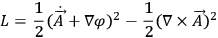
 defines a field of plane surfaces on which the pseudo-metric
 vanishes.
“(4) By introducing an extra dimension, one can have a Lagrangian corresponding to a Riemannian pseudo-metric (degenerate quadratic form), and it seems that the explicit calculations in the classical part could then be simplified.”
ANDERSON and LAURENT
The chief difficulty in this procedure rests in the fact, of course, that one of the equations of motion for the field is free of second time derivatives and therefore represents a restriction on initial and final values which one may impose on the field conditions. However, if one transforms to a set of field variables which include
 ,
,
 , and the scalar field
 , then the equations of constraint do not depend on
 . In fact, the Lagrangian originally looks like
|
and the equations of constraint appear as
|
so in terms of
 ,
,
 ,
,
 equations of constraint
|
Thus solutions satisfying all field equations yield for

|
Thus the construction of the Feynman integral is then seen to be in terms of
 alone, and the measure is given uniquely by the Lagrangian - in this case simply 1.
If one were to extend this line of reasoning to the gravitational case, it is seen that one must look for a set of variables which have the property that they do not appear in the constraint  which corresponds in the electromagnetic case to the scalar potentials. The elimination of the longitudinal part of the gravitational field is of course a much more difficult
problem and has in no way been solved as yet, although it appears to be the central problem to the quantization.”
which corresponds in the electromagnetic case to the scalar potentials. The elimination of the longitudinal part of the gravitational field is of course a much more difficult
problem and has in no way been solved as yet, although it appears to be the central problem to the quantization.”
LAURENT
“In the following I wish to explain why I think that it is worthwhile to try Feynman's action method
I shall start with the simplest generally covariant theory known, that is electrodynamics, which is covariant with respect to gauge transformations.
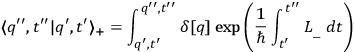
Feynman's
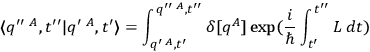
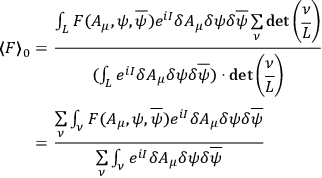
|
21.1 |
Here
 is the action-functional for the fields (or field) and all
 stand for the field-functions in the
 space-time points
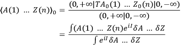
 . The integrals are functional integrals over the functions in all space-time, performed after a certain small imaginary term has been added to the action (as Burton and DeBorde show, this picks out a vacuum state). An extended class of operators may be constructed as sums of time-ordered products
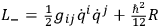
 . To be general I shall in the following write
 instead of
 in (21.1).
 is here a functional of the fields
 .
.
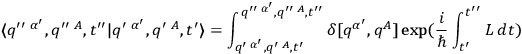
In the usual Lorentz-gauge electrodynamics a vacuum propagator is to be written as follows:
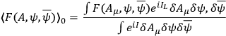
|
21.2 |
A special device must here be used to obtain the wanted anticommuting properties of
 ,
,
 7
7
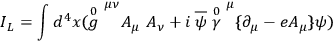
|
21.3 |
where
 is the Lorentz-metric and
 the Dirac-matrices.
(21.2) is exactly the ordinary vacuum propagator of electrodynamics if we restrict
 so that we have nothing but electrons and transversal photons in the initial and final states.8
 may for instance have the following form:

|
21.4 |
Here
 is a normalizing factor
 and
and
 .
.
The operator corresponding to (21.4) gives merely transversal photons in the initial and end states of the propagator.
Observe that in a gauge-transformation
|
21.5 |
 in (21.4) is invariant. We shall assume throughout that our
 's have this property.
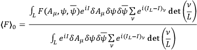
Let us now re-form (21.2)
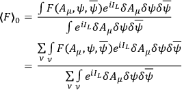
|
21.6 |
We have split up the integrals over all possible
 -functions in sums of integrals over part-regions, of which the first is around the
 -functions satisfying the Lorentz-condition. The other regions are obtained from the Lorentz-region by gauge-transformations. The regions cover completely the region of all
 -functions and they do not overlap. The part-regions can be made as narrow as we like.
Remembering that
 is invariant and that the gauge-transformation is linear we see that the following is true:
|
21.7 |
 is the complete gauge-invariant action
|
21.8 |
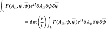
 is the Jacobian of the transformation from the
 -th region to the Lorentz-region. In this case
 is 1 but we shall keep it in in spite of that to be able to use the result later in gravitation theory.
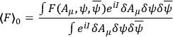
We may now write
|
21.9 |
 depends on the region only (when the region is narrow). In the Lorentz-region,
 . Hence
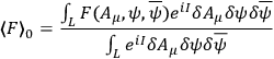
|
21.10 |
Further we see that
|
21.11 |
|
21.12 |
From this form it is evident that the propagator is invariant.
We see from this that under the supposition made about
 , that it must not change its form when
 is replaced by
 , the two demands are fulfilled that quantization shall, as in (21.10), be performed over the “real degrees of freedom” only and that the procedure shall be covariant as in (21.12).
According to the foregoing it is close at hand to guess that a propagator in a theory that is covariant with respect to linear transformation shall be written in the form (21.12), where
 and
and
 must be invariant in the sense mentioned above9
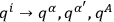
 10 (in the general case we call it extended gauge-invariance). If in gravitation theory, for instance,
 is a functional of the
 only it must not change its form in the linear transformation
 ,where
 is an arbitrary (non-singular) transformation. We observe that a scalar does not necessarily fulfill the requirement, because, in general, it changes its functional form of
 in the transformation. If
 is a function as here described and the integration variables transform linearly, we see from the procedure followed in the electromagnetic case that we may always come from the covariant propagator of type (21.12) to the propagator of type (21.10) , where only so much of the field is quantized as there are “degrees of freedom.”11
A difficulty in the gravitation case is that we do not know over which variables we ought to integrate, and which measure should be chosen in the functional integral.12
The choice of integration variables that seem most natural at first sight is perhaps that of the
 or
or
 , but as Professor J. A. Wheeler
(MISNER
Finally I should like to say a few words about how functionals of the type mentioned earlier may be constructed in gravidynamics.13 Integrals of scalar densities over all space-time is of this type but they do not seem to be of much use in this connection. Professor O. Klein has pointed out to me that the total energy-momentum pseudo-vector may be useful here, and in fact we see that it is of the correct type if we choose it in the following form:
|
21.13 |
(I do not think that this formula needs any explanation.)
 is identically satisfied which gives (21.13) the desired property for
 -transformations which are identity-transformations on the boundaries of the integration-volume. Now all the propagators in the foregoing are limits when the space-time region involved becomes infinitely large14 and nothing hinders us from prescribing, for instance, the Lorentz-metric outside the region and on its boundaries. This means that every interesting transformation is of the type mentioned. In this case the propagator is dependent on the boundary conditions chosen in infinity.”
During the discussion which sandwiched and followed LAURENT's - FEYNMAN raised the difficulties brought in by the presence in
 , of second derivatives.
BELINFANTE
FEYNMAN defined by the equation
 )? More precisely, what is the expression of the determinant which gives a value to the path integral independent of the mesh introduced for its definition?
WHEELER in electrodynamics) and of the true (or physical) variables (such as
 ). At present we have three schemes:
– “Sum over fields” expressed in terms of latent variables. The infinities cancel out.
– Add a term to the Lagrangian so as to make the problem non-singular.
– Use only physical variables.
The whole art is working back and forth between latent and true variables. It is important to show the equivalence of the various schemes and to show the equivalence of the various “slicings,” but it is a task yet to be accomplished.
BERGMANN
One word about why the two approaches appear to lead to mutually consistent results in electrodynamics: in electrodynamics the components of the metric tensor, that is the second derivative of the Lagrangian with respect to the velocities, are constants. It appears natural that in such a situation there should be no disagreement; but I feel very doubtful, without availability of further strong arguments, about anticipating a similar agreement in general relativity, where the same coefficients are complicated functions of the field variables.
I think it is obvious to all of us that the difference between the two approaches again amounts to an estimate of the relative importance of true observables vs. all dynamical variables. Therefore, permit me to give one more argument
that indicates the probable importance of the true observables, or dynamical variables as John Wheeler
I would like to close with a comment on the motivation for Feynman quantization -number theory, and examining the intrinsic structure of a full-blown covariant
 -number theory.”
Footnotes
Feldquantisierung, lecture notes, Zürich, 1950-1951.
J. H. Van Vleck. Proc. Nat. Acad. Sci. 14, 178 (1928); C. Morette. Phys. Rev. 81, 848 (1951).
Can. J. Math. 2, 129 (1950).
Nuovo Cimento IV, 1445 (1956).
R.P. Feynman: Rev. Mod. Phys. 20, 367 (1948).
P. T. Matthews, A. Salam: Nuov. Cim 2, 120 (1955); W. K. Burton, A. H. DeBorde: Nuov. Cim 4, 254 (1956); P. W. Higgs: Nuov. Cim 6, 1263 (1956).
Feynman, op. cit., and Burton and DeBorde, op. cit..
Switching off of the electron charge
 is here assumed.
This does not mean that we have no use for other types of
 in intermediate calculations. In electrodynamics with truncated Lorentz-gauge action we may, for instance, calculate (21.2) with
 and that is very useful.
 is not necessarily the classical action-functional for the system (also when such a functional exists), but it should go over into the classical function when
 .
.
 in (
in (In electrodynamics this question is easily answered: Every gauge-invariant functional is of the wanted type. If the gravitational field constant is switched on and off, the matter can to some extent be made equally simple in gravidynamics.
Burton and DeBorde, op. cit.; Higgs, op. cit..