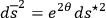
I write for the space-time manifold

|
7.1 |
where I take as the basis in my four-dimensional manifold one vector orthogonal to the initial hypersurface, so that

|
7.2 |

|
7.3 |
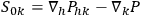
Then the differential relations for the field can be written in the form
|
7.4 |

|
7.5 |
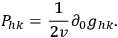
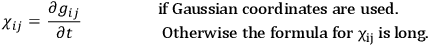
where
 is the covariant derivative, and
 is what Lichnerowicz
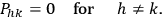
  . (For further notation see Section 5.4 of the talk by Lichnerowicz earlier in this session.) If the coordinates were orthogonal we would have
 , and hence
|
7.6 |
The coefficients
 are the coefficients of the second fundamental quadratic form of the hypersurface
 .
.
We are dealing with the purely gravitational case. To solve the differential equations I choose on the hypersurface three particular vectors, the eigenvector of the tensor
 , that is to say we will have
|
7.7 |
 ,
,
 ,
,
 are unknowns. The metric of the hypersurface
 is
is

|
7.8 |
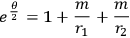
If I set
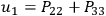 , et cycl., and if I use Lichnerowicz’s
|
7.9 |
then I obtain the following system of equations:

|
7.10 |

|
7.11 |
where
 is the Beltrami operator

|
7.12 |
“It is possible to solve this system of equations which are linear with respect to the highest derivatives. For instance, I can solve them by giving the values of the unknown
 in my three-dimensional space
 on a two-dimensional variety
 , and I can solve then the Cauchy
  . A general iteration method can be used to solve the set of equations by writing them in the form of integral equations using Green’s functions.
  on the boundary, and the values of the
 on
on
 , then I find the general solution of these equations. This is a rigorous mathematical treatment of the problem of initial values.”
WHEELER yields
 in all space if it is known over a two-dimensional surface. However, one would still like to have a potential which gives the field automatically without having to do any integration.
MME. FOURES,
DE WITT asked if the Cauchy
MISNER  you put
|
7.13 |
 and
and
 being distances measured from two points in space. Then you assign initial conditions for the eigenvalues
 . You want to specify
 in such a way that the
velocities of the two particles are initially like that:
in such a way that the
velocities of the two particles are initially like that:

|
Then you try to use the same method which was used for the general proofs to find particular solutions not just on
 but through all space. These can be interpreted as two particles which are non-singular, or they can be thought of as the kind of
 type singularity of which one ordinarily thinks in gravitational theory. These partial differential equations, although very difficult, can then in principle be put on a computer.”
DE WITT pointed out some difficulties encountered in high speed computational techniques. “Singularities are of course difficult to handle. Secondly, any non-linear hydrodynamic
BERGMANN
ANDERSON  do not appear, just as the time derivative of the scalar potential does not appear in the electromagnetic Lagrangian, it may be possible to break up
 in a fashion analogous to the separation of the vector potential in the electromagnetic case into transverse and longitudinal parts. Only one of these parts appears in those equations of motion which are free from second time derivatives. One could then initially and finally specify the part which does not appear in these equations, and obtain a complete solution. There may be one catch to this. There is reason to believe that one of the field equations, which do not depend on second time derivatives, is really the Hamiltonian of the theory.
If that is the case one would not be allowed to specify independent initial and final values for the quantities just discussed.
in a fashion analogous to the separation of the vector potential in the electromagnetic case into transverse and longitudinal parts. Only one of these parts appears in those equations of motion which are free from second time derivatives. One could then initially and finally specify the part which does not appear in these equations, and obtain a complete solution. There may be one catch to this. There is reason to believe that one of the field equations, which do not depend on second time derivatives, is really the Hamiltonian of the theory.
If that is the case one would not be allowed to specify independent initial and final values for the quantities just discussed.
Discussion of these points, which are closely related with the problem of quantization, was postponed until later.
WHEELER
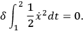
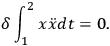
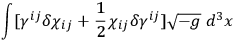
“I would like to raise in this connection the question of the use of the variational principle itself. The variational principle in general relativity
|
7.14 |
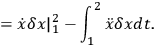
How do we tell what to fix at the endpoints of the time interval? We do this by performing an integration by parts:
|
7.15 |
From this we draw two separate conclusions:
1 .
.
2 at the two endpoints of the motion, i.e., we must specify the coordinate
 at the times 1 and 2. This is a time-symmetric specification. One is so accustomed to this pattern of thinking that when general relativity presents us with a different pattern we are not prepared for that. Therefore, let me introduce a problem which does have the pattern characteristic of general relativity, and let us see how we would face up to it.
Consider this:
at the times 1 and 2. This is a time-symmetric specification. One is so accustomed to this pattern of thinking that when general relativity presents us with a different pattern we are not prepared for that. Therefore, let me introduce a problem which does have the pattern characteristic of general relativity, and let us see how we would face up to it.
Consider this:
|
7.16 |
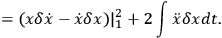
Traditionally one abhors these second derivatives in the problem, so one quickly transforms it into the previous problem. I propose to deal rather directly with the new problem like this:
|
7.17 |
The conclusions would now be:
1 .
.
2 ,
i.e., we are to specify the value of
,
i.e., we are to specify the value of
 at the two endpoints of the motion.
“In other words, we are led here to a different kind of specification of the problem. I merely want to point out that the variational problem itself has the property if we don’t monkey with it, to tell us what it is that we should deal with.”
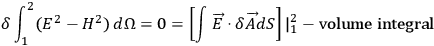
“In the case of electromagnetism we can also let the variational principle tell us what the quantity is that we are concerned with. Note the equation:2
|
7.18 |
The volume integral gives us the usual field equations. The boundary term tells us that we should specify
 at the limits. If you specify
 itself, rather than its transverse part, you would be taking too seriously the demand that the boundary term must vanish. Clearly you don’t have to be that hard on
 . Analogous considerations can and have been applied to the general relativity by Misner
MISNER  in the sense mentioned by Wheeler.
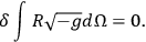
|
7.19 |
From this one gets the surface term of form:
|

|
|
The suggestion is that if you look at the surface term carefully you will find what the correct variables to use are, and what you can specify on the initial and final surface.”
MISNER  and
and
 at some initial surface, say at
 . Now, if you don’t watch out when you specify these initial conditions, then either the programmer will shoot himself or the machine will blow up.
  at the initial time. These are what are called the “constraints.”
  . They are the equations to which we have been finding particular solutions; and on the other hand, Mme. Fourès has shown the existence of more general kinds of solutions. Mme. Fourès
LICHNEROWICZ is compact and whether
 is orientable.